Abstract
ASTM Test Method E 112 says it covers test methods to determine the average grain size of specimens with a uni-modal distribution of grain areas, diameters or intercept lengths. It says that these distributions are approximately log-normal. But, it does not describe how one can determine if their specimen’s grain size distribution is a uni-modal normal (Gaussian) distribution. ASTM E 1181, Standard Test Methods for Characterizing Duplex Grain Sizes, says it covers test methods to characterize grain size in products with any other distribution (other than a “single log-normal distribution of grain sizes”). But, the only example given in Appendix X2 shows the percentage of the number of intercept measurements in 38 length classes from 0 to 1 to 37 to 38 mm. Thirty eight classes is far too many to properly reveal the grain size distribution. This procedure reveals a log-normal distribution but it is not in terms of ASTM grain size numbers, which makes it less useful.
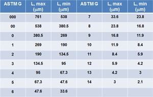 |
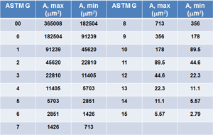 |
| Table 1: Binning of Linear Intercepts by G Class | Table 2: Binning of Grain Areas by G Class |
Introduction
In the introduction of E1181, it says that “the term ‘duplex grain size’ is chosen to describe any of these other distributions (other than uni-modal) of grain size, because of its common usage and familiarity.” But, while this may be a commonly used term by some, it is not correct. All non-uni-modal normal, Gaussian distributions are not duplex grain size distributions. Two general types of classifications are given: a random duplex grain size and a topological duplex grain size distribution. The random duplex grain size classification has two sub-categories: a “wide-range” condition and a “bi-modal” condition while the topological duplex grain size classification has three sub-categories: a “cross-section” condition, a “necklace” condition; and, a “banded” condition.
Procedure
So, how do we evaluate grain size distributions? We measure grain areas or lineal intercept lengths and then calculate the skew and kurtosis of the data. All distributions will have a positive skew due to the fact that grain measurements are made on a two-dimensional sectioning plane through a three-dimensional microstructure. This produces grain areas or intercepts of a single grain varying from the maximum dimension to a very small dimension. A kurtosis <5 indicates a normal uni-modal distribution, with a value of 3 being a perfect normal distribution. Next, order the L or A values from highest to lowest and then add up the total length or total area as a function of G limits (see Tables 1 and 2). Then, plot the % intercept length or % grain area as a function of the G class (x-axis) to see the shape of the distribution curve.
To define a “normal” distribution, plot the area percentage of grains per ASTM grain size class. The definition of G according to E112 is:
NAE = 2G-1 (1)
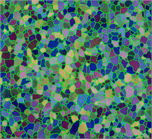
where NAE is the number of grains per square inch at 100X and G is the ASTM grain size number. Figure 1 shows the equiaxed grain structure of a motor lamination sheet steel color etched using Klemm’s I reagent. Figure 2 shows the detection of the grain boundaries using the Thixomet image analyzer. This image can be inverted to detect the grain interiors and then measure the area of each grain. The grain areas were used to calculate the skew and kurtosis revealing a skew of 1.43 and a kurtosis of 2.55 for 891 grains measured. The mean grain size is 6.63. The kurtosis shows that this is a normal, uni-modal, Gaussian grain size distribution.
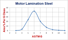
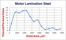
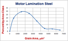
The grain areas are then ordered from largest to smallest and then the areas in each ASTM G class, as defined in Table 2, are calculated. Then, for each G class, divide the sum of the grain areas by the total grain area and express this as a percentage. Then, plot on the x-axis the ASTM grain size, G, and on the Y-axis, the area percentage of grains per G class, as shown in Figure 3. Table 3 lists a summary of the data used to create Figure 3. Figure 4 shows plots of area classes in μm2 on the x-axis and the area % per class on the y-axis using 14 versus 7 classes (far less than 38 classes shown in Appendix X2 in E1181). Note that the use of 7 classes better characterizes the nature of the log-normal relationship than 14 classes. Classing the grain areas according to the ASTM G value converts the log-normal relationship into a normal relationship due to the definition of G in equation 1.
 |
| Table 3: Percentage of Grains by Area Per G for the Motor Lamination Steel
|
Conclusion
Before we can define non-normal distributions, we must define what a normal, or Gaussian, uni-modal distribution is and how we can determine that it is such. The example illustrated, according to the definitions in E1181, paragraph 8.3.1.2, claims that this is a wide-range duplex grain size distribution because it covers 8 grain classes, which is greater than 5 classes, as in the definition given in 8.3.1.2. Plotting the area % of grains against the ASTM grain size number, G, converts the log-normal distribution, obtained if grain areas are plotted on the x-axis, into a normal distribution. The shape of the distribution curve is clearly normal and uni-modal and the kurtosis was 2.55, proof of a normal distribution.
George Vander Voort has a background in physical, process and mechanical metallurgy and has been performing metallographic studies for 48 years. He is a long-time member of ASTM Committee E-4 on metallography and has published extensively in metallography and failure analysis. He regularly teaches MEI courses for ASM International and is now doing webinars. He is a consultant for Struers Inc. and will be teaching courses soon for them. He can be reached at 1-847-623-7648, EMAIL: georgevandervoort@yahoo.com and through his web site: www.georgevandervoort.com
To View a listing of all George’s articles please click here
Read George Vander Voort’s Biography


